Noise bridge measurement case study - shortened vertical monopole matching

Charley, K1DNR, has a nominally 40m quarter wave vertical monopole, ground mounted with buried radials and fed with about 30m of LMR-400, and enquired about its use on the low end of 80m.

Problems

The 40m quarter wave vertical monopole at 80m will be about λ/8 electrical length, and have a relatively low feed point resistance and fairly high capacitive reactance. This leads to the following issues:

the equivalent radiation resistance would probably be a small part of the feed point resistance, and so gain will be degraded somewhat, perhaps 5dB or so over a quarter wave vertical;
directly fed with coax, loss on such a feed line will be quite high, possibly some 5 to 15dB for 30m of LMR400, and worse for poorer cables such at RG58; and
the impedance looking into the feed line is unlikely to suit the transmitter, and an ATU will probably be required, accounting for some further loss, perhaps a few dB.

A solution

Baseline

The high feed line and ATU loss can be reduced markedly by performing impedance transformation at the feed point.

So the first step in the design process is to quantify the actual load impedance to be transformed.

Fig 1: MFJ202B
(Picture courtesy of K1DNR)

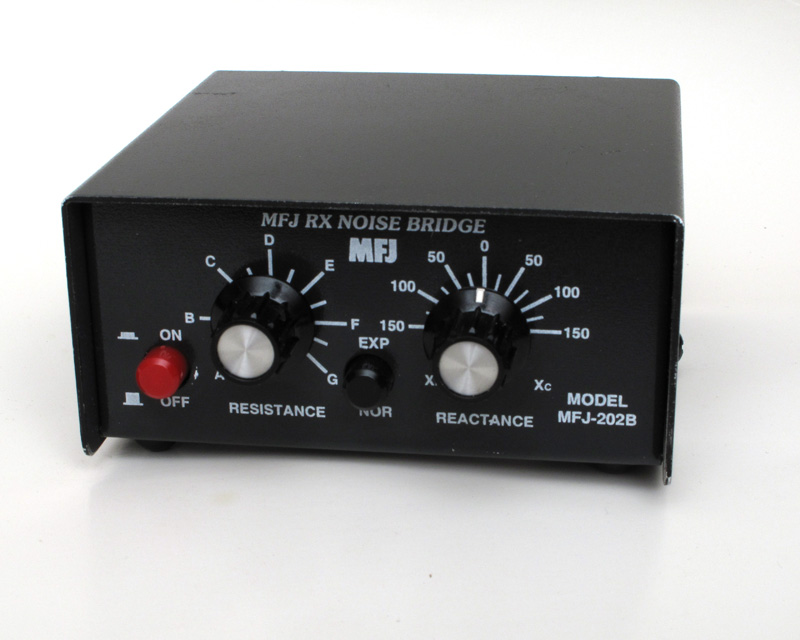
Fig 1 shows the MFJ-202B Noise Bridge. Note the sparsity of scale graduations makes precise reading very challenging.

The impedance right at the antenna base was measured using a MFJ202B noise bridge. Importantly, the connection from the radials to the coax shield was maintained so that the common mode current path provided by the coax was not any different to the normal operating configuration. This means the coax was connected right through to the transmitter in the normal way.

The first round of measurements when plotted demonstrated the extreme sensitivity of calculated R and X values to the dial readings from the noise bridge, and drove a second round of more careful measurement.

A spreadsheet was prepared to calculate key metrics from the dial readings. The spreadsheet provided a function to perform a cubic spline interpolation of R dial readings entered as a.dd where a was the dial letter, and dd a decimal interpolation of the dial setting between lettered graduations using MFJ's supplied calibration data.

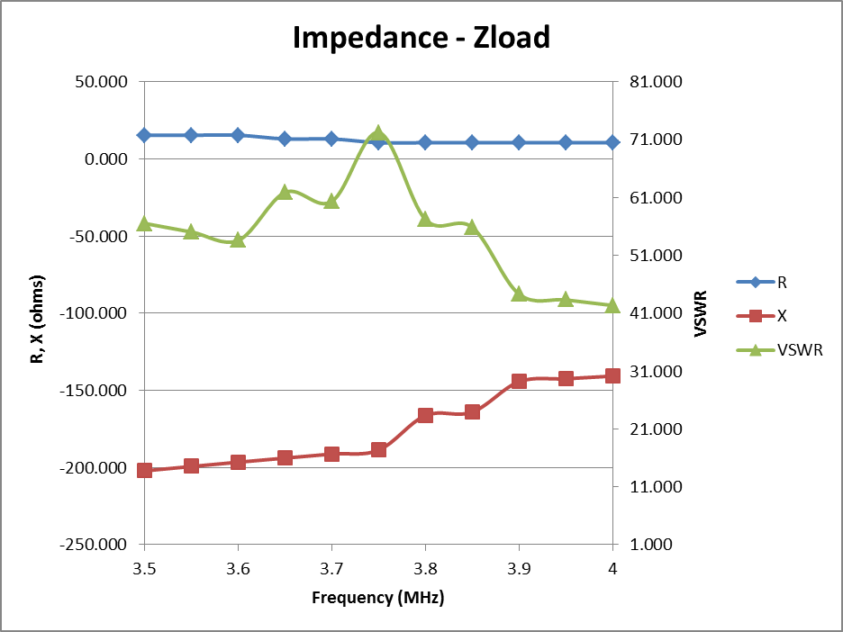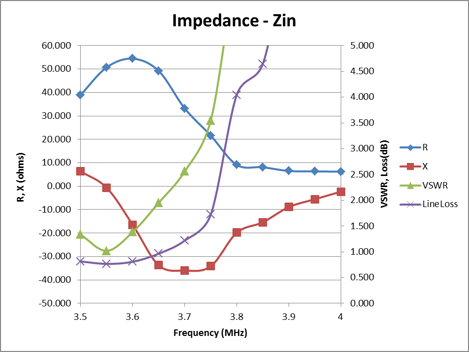
Fig 2: Baseline - feed point impedance

Fig 2 shows the calculated impedance and VSWR(50) at the antenna feed point across the 80m band. There is obviously a bit of measurement noise, but the measurements:

confirm the R is varies slowly across the band;
give a figure of around 15Ω at the target operating frequency;
confirm that X varies more quickly with frequency;
gives a figure of around 200Ω capacitive reactance at the target operating frequency.

Before moving on with the design, it is worth examining line input impedance and loss in the unmatched configuration.

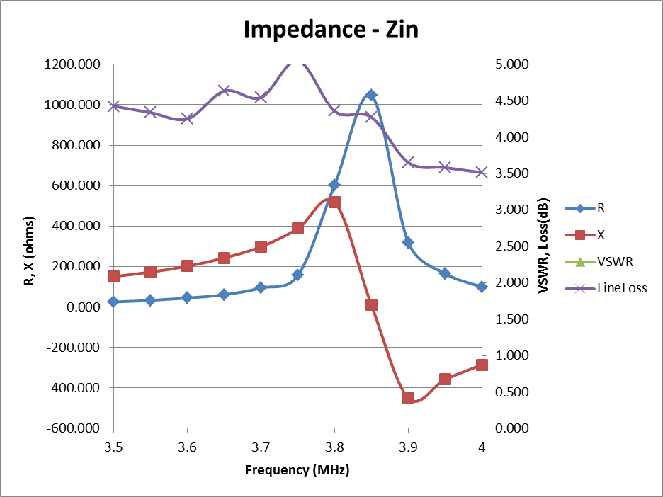Fig 3: Unmatched and using 30m of LMR400 feedline

Fig 3 above shows a rapid change in impedance around 3.8MHz which is cause by the fact that at that frequency, the end of the line is in the region of a voltage maximum. The impedance figures could be used to model the loss in a typical ATU, and in this case, less than 1dB at 3.55MHz (though significantly worse at the high end of the band). So, the main issue is around 4.5dB of line loss in the mismatched state.

Matched

Knowing the feed point impedance, a simple L network was designed to transform it to approximately 50+j0Ω. The network is a low pass with shunt C of 1277pF on the source side of the 10µH inductor (Q=200).

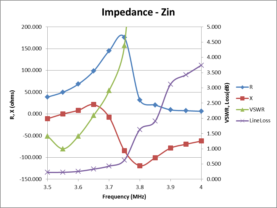Fig 4: Matched and using 30m of LMR400 feedline

Fig 4 shows impedance and VSWR at the source end of the feed line with the L matching network tuned for 3.55MHz. VSWR is less than 1.5 for more than 100kHz, and line losses are less than 0.3dB below 3.6MHz. At ATU could be used to mop up the small impedance variation at the low end of the band, and losses will be very low.

The solution with matching network at the antenna feed point will be about 5dB higher gain than direct coax feed. The difference would be greater if higher loss coax (such as RG213 or RG58) were used.

Fig 5: Matched and using 30m of RG58C/U feedline

In fact, once the high VSWR of the unmatched solution is eliminated, the need for low loss coax is much less. Fig 5 shows the same data for the case of 30m of RG58C/U. In this case, coax loss at 3.55MHz is less than 0.6dB worse than the much more expensive LMR400. (The matching network was the same as in Fig 3, it was not optimised for RG58C/U.)

Spreadsheet tool

Fig 6: Matched and using 30m of RG58C/U feedline

Fig 6 is a reduced screen shot of the spreadsheet developed to support the design task. Click on the image for a full sized picture. You may then need to click on the resultant image to expand it to full resolution, albeit possibly with scroll bars.

The L network was optimised using Excel Solver to find L and C for minimum VSWR at line input at 3.55MHz.

Conclusions

The humble noise bridge (in this case an MFJ202B) in capable hands can provide a very useful tool for antenna system design projects, though it takes experience and knowledge and a great deal of care to make valid measurements. Augmented by some spreadsheet calculation and presentation tools, the data is clear in guiding design direction.

The MFJ-202B has quite small scale length, and lacks fine graduations, so reading it to high accuracy is challenging.

Changes

Version	Date	Description
1.01	06/10/2011	Initial.
1.02
1.03