A graphical explanation of energy flow in a practical transmission line

Introduction

This article examines steady state energy flow in a practical mismatched line scenario.

The load case and line parameters are chosen to make the example a simple one that is clear in the graphs, and easily grasped, but the example is also a very practical one, and the analysis and explanation does not depend on assumptions of a lossless line.

Key model characteristics are:

the frequency is 7.060Mhz;
the load impedance is chosen to be 56-j72Ω, and is typical of that which might be obtained from a shortened half wave dipole near ground;
the transmission line is 12m of RG58C/U (characteristics taken from TLLC); and
the source supplies 100W average power to the line.

The analysis is performed using the Telegraphers Equation.

Definitions

'Steady state' means continuous sinusoidal excitation (at a single frequency), and after sufficient time that the system has settled.

'Mismatched line' means that the load impedance is different to the characteristic impedance of the transmission line.

'Power' is the rate of flow of energy.

Conditions at the source

The model has been chosen so that the impedance seen by the source is 150+j0Ω, or 150Ω purely resistive.

Fig 1: Conditions at the source

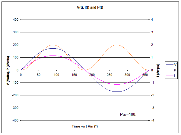
Fig 1 shows the instantaneous voltage, current and power at the source end of the line. The time axis is scaled in time in electrical degrees, and a full AC cycle is shown.

Note that I is in phase with V, in fact I is V/150. A consequence is that instantaneous power which is voltage times current varies (the P curve), but is NEVER negative, ie there is NEVER a flow of energy towards the source, not even for an instant. The power averaged over a full AC cycle is 100W.

If you were to measure the VSWR at this point, it would be 3.0.

Conditions at 5m from the source

Fig 2: Conditions at 5m from the source

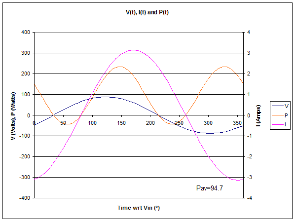Fig 2 shows the instantaneous voltage, current and power at 5m from the source end of the line. The time axis is scaled in electrical degrees wrt V at the source end, and a full AC cycle is shown. I is not in phase with V, it lags V. There are some times when the instantaneous power is negative, ie energy flows towards the source.

Note that in Fig 2, power is negative (energy flows towards the source) from time=35° to 80°, yet at the same time Fig 1 shows power at the source as positive (towards the load). How can this be?

The instantaneous power plot at this point is not identical to that at the source because energy is stored in electric and magnetic fields in the transmission line, and under mismatched conditions, energy is exchanged between sections of line, and possibly between load and line and line and source. At some instants, the power is greater than in Fig 1, energy that was stored in the line section is flowing towards the load, at some other instants, power is less than in Fig 1 and energy is being stored in the line section.

Note that the average power remains positive, over the full AC cycle there is a net energy flow towards the load, though in this case, it is less than the power input to the line due to line losses.

Note also that voltage is a good deal lower than at the source, and the current is considerably higher. It is the ratio of voltage to current (considering their phase) that gives the impedance at this point, and it is 19+j20Ω. Impedance varies along a mismatched line as a consequence of the standing waves.

If you were to measure the VSWR at this point, it would be 3.2.

Conditions at 9m from the source

Fig 3: Conditions at 9m from the source

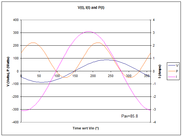Fig 3 shows the instantaneous voltage, current and power at 9m from the source end of the line. The time axis is scaled in electrical degrees wrt V at the source end, and a full AC cycle is shown.

Compare Fig 3 with Fig 2. Note the times when power is negative, they are different in each case.

The magnitude of V and I are similar, but the phase is different, and Z in this case is 18-j22Ω.

Average power is even lower, a consequence of line loss. Note that 5.3W was lost in the first 5m of line, then the 4m of line from 5m to 9m accounts for 8.9W. More power is lost in the region of a current maximum in the standing wave pattern in most practical transmission lines at HF, and the current maximum is at 7m from the source in this case.

If you were to measure the VSWR at this point, it would be 3.3.

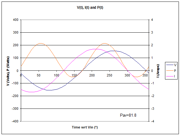Conditions at 12m from the source (at the load)

Fig 4: Conditions at 12m from the source (at the load)

Fig 4 shows the instantaneous voltage, current and power at 12m from the source end of the line. The time axis is scaled in electrical degrees wrt V at the source end, and a full AC cycle is shown.

The instantaneous power is negative at times. Energy is exchanged between the line and load, but there is a net average energy flow of 81.8W.

The ratio of V to I (considering phase) again gives us impedance, Z=56-j72Ω.

Average power is even lower, a consequence of line loss. Note that 5.3W was lost in the first 5m of line, the the 4m of line from 5m to 9m accounts for 8.9W. More power is lost in the region of a current maximum in the standing wave pattern in most practical transmission lines at HF, and the current maximum is at 7m from the source in this case.

If you were to measure the VSWR at this point, it would be 3.5. VSWR decreases smoothly from load to source for most practical cases at HF, and the decrease is accounted for exactly by line loss.

Field implications

If you can visualise that the transmission line has sinusoidal current and voltage at every point along the line, the current and the voltage are due to the sum of the components due to the forward and reflected waves, the phase relationship of current and voltage vary with each other, and with displacement along the line. Associated with each sinusoidal voltage is a sinusoidally varying electric field, and with each sinusoidal current, and sinusoidally varying magnetic field. Energy is flowing in a cosine pulsating fashion at twice the frequency of the voltage or current, and energy may be flowing in one direction and sometimes in another at different points along the line, but at every point along the line, there is an average flow of energy towards the load (albeit smoothly decreasing towards the load due to line loss).

If a line is sufficiently long, there are points where V and I are in phase, and these points occur every half wavelength (electrically). At these points, there is NEVER energy flow towards the source, not even for an instant. Yet at points in between, there can be instantaneous energy flow towards the source, so these points demarcate boundaries of regions of interesting cyclic energy exchange whilst supporting net energy flow from source to load.

It is indeed a complex multidimensional picture, which probably accounts for why it is often not well understood.