| OwenDuffy.net |
|
*** DRAFT ***
So called pipe cap filters find application in the GHz range in ham receivers and transmitters. Judging from posts in online fora, there is some confusion about how the things work, and how to optimise them. This article explores some of the issues with a single pipe cap filter using a theoretical model.
Before delving into the device, lets review the meaning of some terms that are relevant to the discussion.
Insertion Loss is defined (FS-1037C 1996) as: [t]he loss resulting from
the insertion of a device in a transmission line, expressed as the reciprocal of
the ratio of the signal power delivered to that part of the line following the
device to the signal power delivered to that same part before insertion
. It
is wrong to assume that Insertion Loss implies conversion of any or all of the
available energy to heat.
(IEEE 1988) defines Return Loss as:
(1) (data transmission) (A) At a discontinuity in a transmission system the difference between the power incident upon the discontinuity. (B) The ratio in decibels of the power incident upon the discontinuity to the power reflected from the discontinuity. Note: This ratio is also the square of the reciprocal to the magnitude of the reflection coefficient. (C) More broadly, the return loss is a measure of the dissimilarity between two impedances, being equal to the number of decibels that corresponds to the scalar value of the reciprocal of the reflection coefficient, and hence being expressed by the following formula:
20*log10|(Z1+Z2)/(Z1-Z2)| decibel
where Z1 and Z2 = the two impedances.
(2) (or gain) (waveguide). The ratio of incident to reflected power at a reference plane of a network.
Return Loss expressed in dB will ALWAYS be a positive number in passive networks.
Transmission Loss is simply PowerIn/PowerOut (irrespective of matching conditions), and it can be expressed in dB as 10log(Pin/Pout).
Q (Qualify factor) is the ratio of energy stored to energy dissipated as heat over one RF cycle.
Postings to online discussions commonly describe one or more of the following problems:
| |
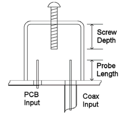
Fig 1 is from (Wade 2008) which gives an outline of how the device operates, proposes an equivalent circuit, and offers some empirically based design graphs.
This article proposes a slightly more complicated equivalent circuit as the basis for discussion of solutions to the common problems discussed.
The device can be thought of as a resonator using three transmission line sections, one formed by the central conducting limb, and the other two being the input and output coupling probes. Properly calibrated, this model ought be more accurate than Wade's lumped component model, particularly at frequencies well above first resonance.
Each TL section operates in TEM mode, but there will be some fringing of electric field in the region around the open ends of each TL section. Each TL section then can be approximated as an o/c line section with some capacitance from the open end to ground to represent the electric field at the ends of the conductors. Further, the coupling probes are inserted into the field created by the central limb, so a small capacitance from the end of each probe to the end of the central limb can approximate that coupling.
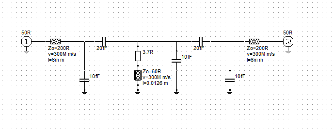 |
Fig 2 shows the topology of the equivalent circuit. The values shown are not based on measurements, but merely reasonable estimates for a filter resonant around 5.5GHz.
The TL sections adjacent to the ports represent the naked probes, and there a small capacitances in shunt with the inboard end to represent 'end capacitance'. The central limb is represented by the middle TL element, the small series R to represent conductor loss. In shunt with the latter is a small capacitance to represent the 'end capacitance'. Two small capacitances couple the probe ends to the end of the main limb.
In an air dielectric resonator, there will be negligible dielectric loss. In this model, the conductor loss in the probes is ignored, they operate at low average current and loss would be low relative to the external cabling. The central limb carries very low current at the open end, and relatively high current at the s/c end, as does the surrounding pipe cap. The small equivalent R in the model is to capture the effect of I^2R loss distributed on the central limb and the adjacent cap surfaces.
Ideally, the model should use a lossy line model for each of the transmission lines. RFSim99 does not support a lossy line model, so the fixed R to represent loss at the resonant frequency is a measure to calibrate the model for loss at that frequency, but the value of the equivalent R is actually frequency dependent and the model accuracy would be better with a tool that supports a lossy line model. Nevertheless, the simple model provides valuable insight.
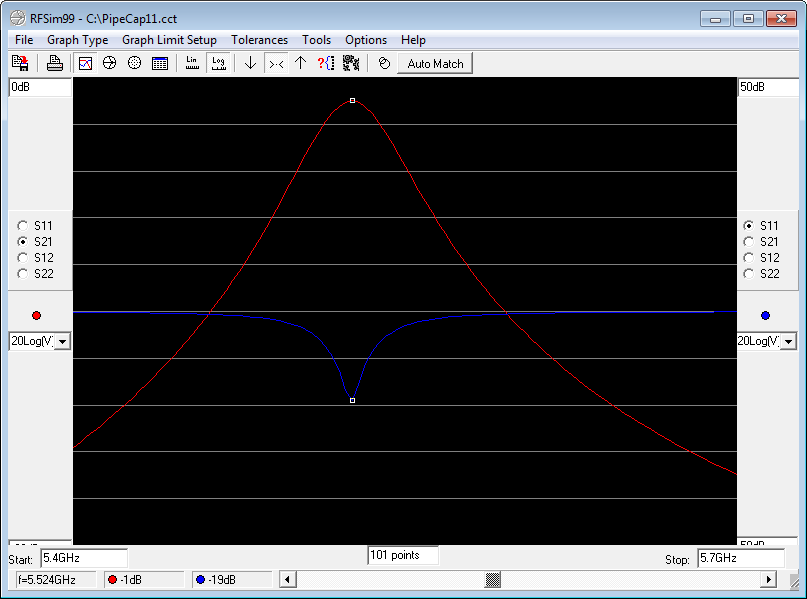 |
Fig 3 shows the response of the model. Return Loss (derived from S11) is very good (19dB), and Insertion Loss (derived from S21) is 1dB. The model is deliberately symmetric, and since it is quite lossy, Return Loss is not very high. Return Loss can be improved by increasing the coupling cap on the left side. Alternatively, reducing the R will improve efficiency and hence Return Loss.
This model allows exploration of in-band transmission loss, bandwidth and out-of-band rejection.
Some simple relationships:
In the example shown, BW=60MHz so Qw=5525/60=92. Since TransmissionLoss=10^(1/20)=1.122, Qi=846.
In a practical filter, in-band Transmission Loss is dominated by the distributed I^2R losses in the central limb and adjacent cap surfaces. The current is very low at the o/c end, and highest at the s/c end, so measures to reduce R at the s/c end will be of most benefit. These surfaces should be good conductors. Choice of brass or stainless steel conductor, threaded surface, and thread electrical interface all seem compromises compared to a central limb of copper soldered to the resonator end. Larger diameter conductors (ie larger diameter pipe cap and central limb) will reduce R and increase intrinsic (or unloaded) Q.
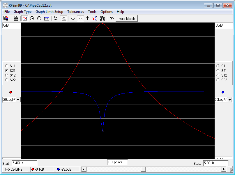 |
Fig 4 shows the effect of reducing R to 0.5Ω, Transmission Loss is reduced to 0.1dB, but bandwidth is almost unchanged.
In-band transmission loss is very sensitive to R, so if the loss in a matched resonator is too high, it is R that is most likely the problem.
In-band transmission loss can be reduced by coupling more tightly, but this will increase bandwidth and reduce out-of band-rejection.
When directly measuring Insertion Loss to assess Transmission Loss, it is vital that Return Loss is sufficiently high that the measured Insertion Loss is mostly due to Transmission Loss.
Bandwidth in a filter with low Transmission Loss is most dependent on the effect of external loading. Tighter coupling increases bandwidth and reduces out-of-band rejection.
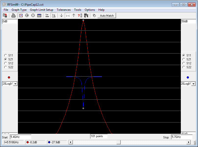 |
Fig 5 shows the effect of reducing the coupling caps to 10fF and retuning (still with the reduced R). Bandwidth is reduced to about 11MHz, and Transmission Loss is quite low at 0.2dB.
As mentioned, loading the device increases bandwidth and reduces loss.
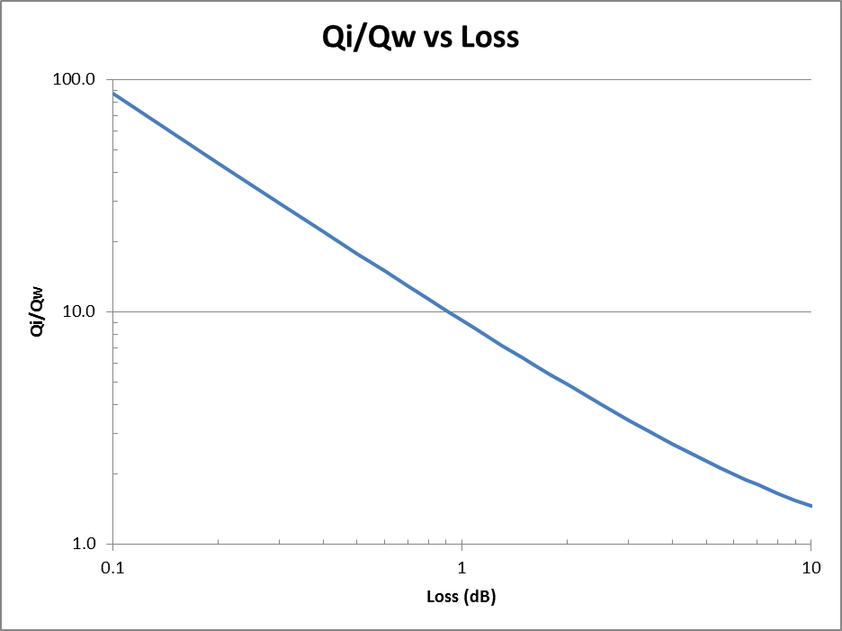 |
Fig 6 shows the relationship between loss and the ratio of Qi/Qw. For loss below 1dB, the ratio Qi/Qw is approximately 9/dBloss.
So, lets say the application requires a 30MHz bandwidth at 3.4GHz, Qw=3400/30=113. Lets say that the filter must have transmission loss of less than 0.5dB, then Qi/Qw must be greater than 9/0.1=90, so Qi must be greater than 1020.
Various commentators have suggested 'normal' losses for these filters, but loss without knowing Qw is quite limited.
(Wade 2008) suggests two to three dB loss for 1% bandwidth as typical. In that case, Qw=100 and Qi=920. Wade opines that Qi between 600 and 1000 is achievable.
(Britain 2008) shows measurements for a 5760MHz filter with bandwidth of about 40MHz and Insertion Loss of 1.32dB. Unfortunately, measured Return Loss is rather poor at about 13dB, so mismatch contributes to the Insertion Loss. If we were to ignore the mismatch, Qw=5760/40=144, Qi=7.2*144=1040. The transmission loss is probably lower than the measured Insertion Loss, and actual Qi is probably a little higher.
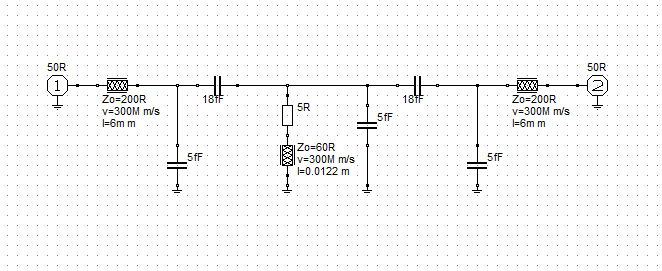 |
Fig 7 shows a model that gives a response quite similar to that reported by Britain for his 5760MHz filter.
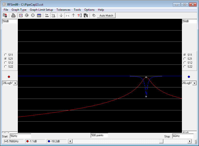 |
Fig 8 shows the model results which compare favourably with Britain's VNA plot for the 5760MHz filter, and could probably be calibrated with a little more fiddling. (The S21 scale is from -50 to +50dB, 10dB per line.)
(K04BB nd) shows measurements of a filter at 2265MHz with 9MHz bandwidth for Qw=251 and measured Insertion Loss of 3dB. He does not give Return Loss, but if we assumed that 3dB was the matched loss, that implies Qi=3.4*251=853.
() shows measurements of a pipe cap filter at 2320MHz with bandwidth of 13.3MHz for Qw=174 and measured Insertion Loss of 2.9dB. He does not give Return Loss, but if we assumed that 2.9dB was the matched loss, that implies Qi=3.5*174=609.
One can't help but think that Qi could be significantly higher than 1000 with attention to reducing I^2R loss in the central limb and adjacent cap surfaces. The theoretical Qi for a long thin optimised air dielectric quarter wave copper resonator is aproximately 8.4*b*f^0.5 where b is the inner radius of the outer conductor. Optimised diameter ratio of inner to outer is 3.6, and 78% of the loss is due to current flowing on the inner conductor. These figures ignore copper loss due to radial currents in the s/c end, so the expected Qi for a short fat resonator will be a little lower. The theoretical Qi for a 20mm diameter optimised air dielectric copper quarter wave resonator at 5500MHz is therefore a little less than 6000, considerably higher than the 600 to 1000 indicated by ham reports. The use of small diameter inner conductor, brass, plated brass, stainless steel etc and threaded conductor surface probably contributes to under achievement.
Mention is made earlier of the limitation of RFSim99 TL models.
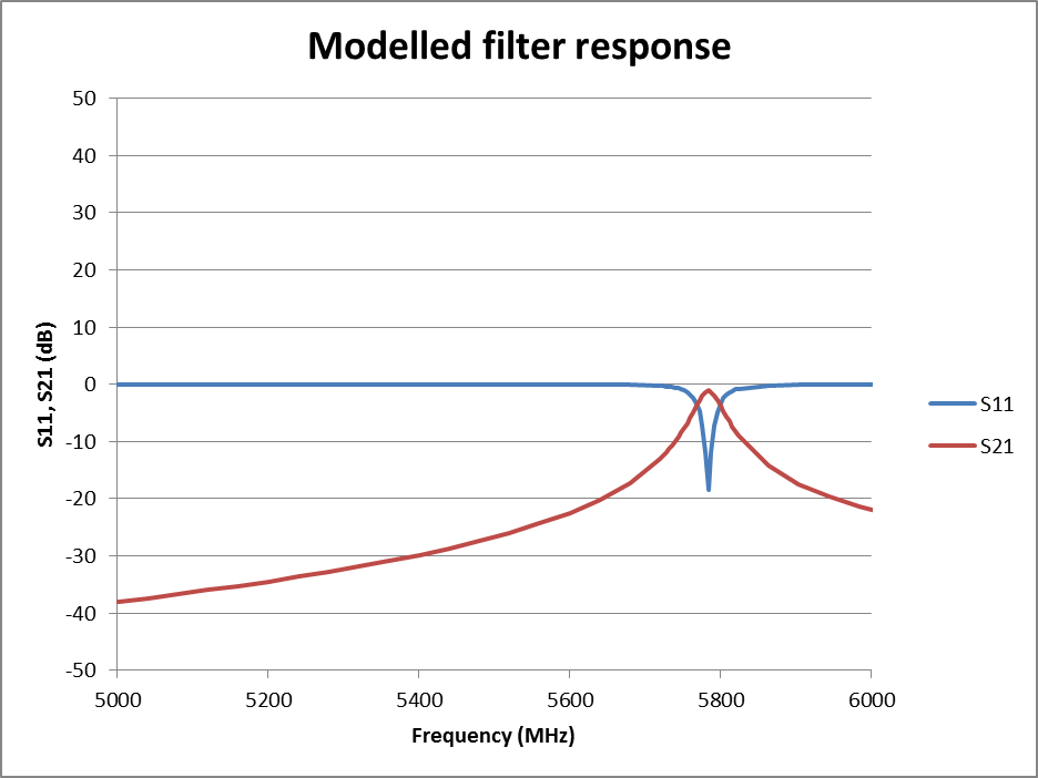 |
Fig 9 shows a lossy TL model of the configuration in Fig 7 with the R omitted. The line loss for the central limb is 5e-6*f^0.5dB/m at 5800MHz. The loss of 0.38dB/m at 5800MHz is greater than that of LDF2-50 Heliax, which suggests that typical constructions may underachieve on Qi.
The model results are similar to that in Fig 8 below resonance, and a little different towards 6000MHz, a little closer to Britain's measurements.
Calculation of more appropriate values for Zo would give a better match to specific applications. For example, a probe using the bare centre conductor of UT-141, 6.35mm offset from centre in a 17mm id pipe cap would have Zo around 125Ω, and a 4mm diameter centre conductor would have Zo around 88 ohms.
If a filter is intended to have low Insertion Loss, then a perfectly matched filter will be almost symmetric. Take a shortcut, and make any changes to coupling symmetrically.
Some designs leave PTFE dielectric on the input and output probes. It is difficult to understand the reason for this, it probably just increases loss.
Adjusting the length of the main limb changes the length of the TL element, changes the 'end capacitance' and changes the coupling... all in one foul swoop. This interaction will make optimal adjustment tedious... especially if the probe coupling position / length cannot be easily adjusted. This probably accounts for most of the difficulty in obtaining good performance.
Conductor loss is probably the greatest source of Transmission Loss in the filter, and that can be reduced by using good conductors, larger parts, smooth conductors, and minimising current flowing through threaded interfaces.
| Version | Date | Description |
| 1.01 | 17/05/2012 | Initial. |
| 1.02 | ||
| 1.03 | ||
| 1.04 | ||
| 1.05 |